Fourier series / May 20, 2026

How Smooth Waves Build Sharp Corners: Making Fourier Series Intuitive

A square wave looks simple. But hidden inside is a stack of sine waves.

A sine wave and a square wave behave very differently. While both are periodic, the sine wave is smooth and curvy while the square wave has an "on and off" behavior.

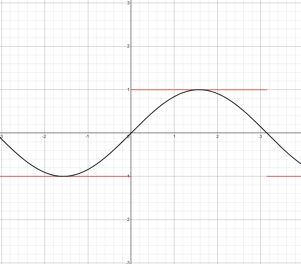
A sine wave and square wave plotted on the same axes. — Sine wave and square wave overlaid

With both shapes in mind, a natural question arises. Is there a way to use the periodicity of the sine wave in order to produce a square wave? This leads us to Fourier's trick, which has underpinned signal processing, circuits, image compression, and so much more since its discovery.

Making The Square Wave

Let's start with the simplest approximation.

S_1(x)=\frac{4}{\pi}\sin(x)

This is our foundation. It does not look like a square wave yet, but it gets the rough shape right:

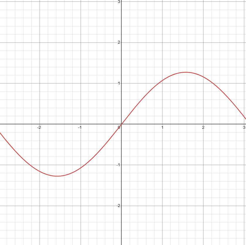
The first sine approximation to a square wave. — $f(x)=\frac{4}{\pi}\sin(x)$

It rises where the square wave rises, and falls where the square wave falls. However, it is still too curvy. For now, think of $\frac{4}{\pi}$ as a scaling factor that makes the height come out right.

Alright, let us add some more approximations by adding the odd harmonics. A harmonic is just a sine wave whose frequency is an integer multiple of the original:

S_3(x)=\frac{4}{\pi}\left(\sin(x)+\frac{1}{3}\sin(3x)\right)

S_5(x)=\frac{4}{\pi}\left(\sin(x)+\frac{1}{3}\sin(3x)+\frac{1}{5}\sin(5x)\right)

The third Fourier partial sum for the square wave. — $S_3(x)$

The fifth Fourier partial sum for the square wave. — $S_5(x)$

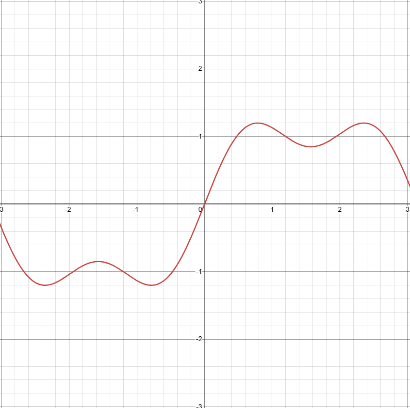
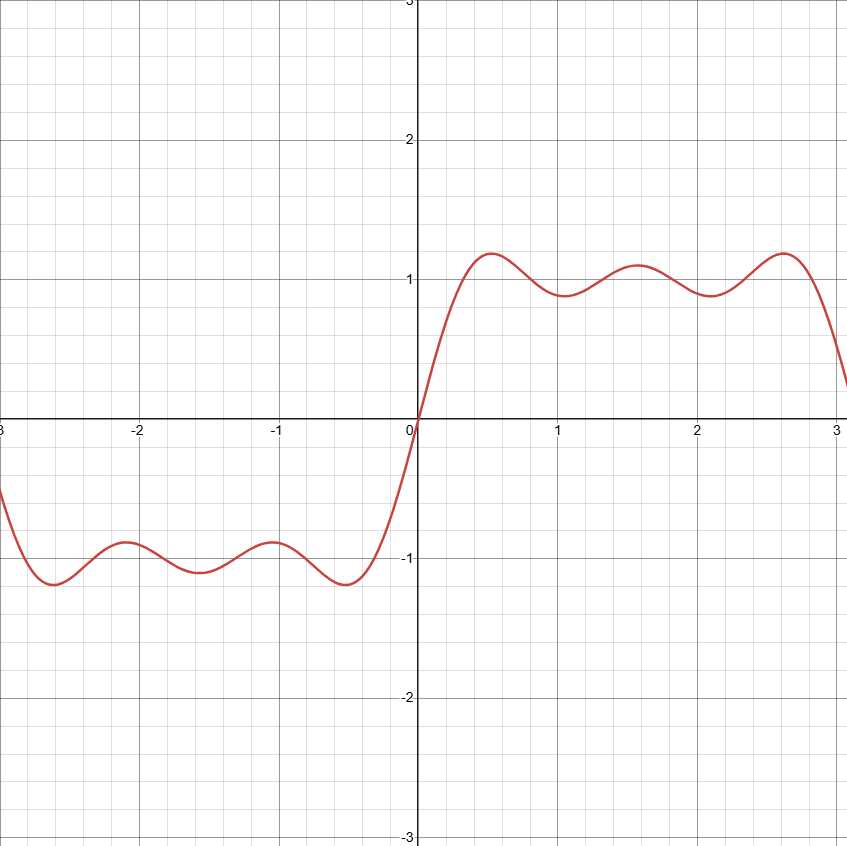
Why are we adding just odd harmonics like this? Each odd harmonic shares a common behavior across $x=\pi,2\pi,\ldots$ . More specifically, each odd harmonic always crosses these points from positive to negative at $x=\pi$ , then from negative to positive, and so forth. Therefore, when all functions are summed, they constructively make a wave that goes from above to below at such points.

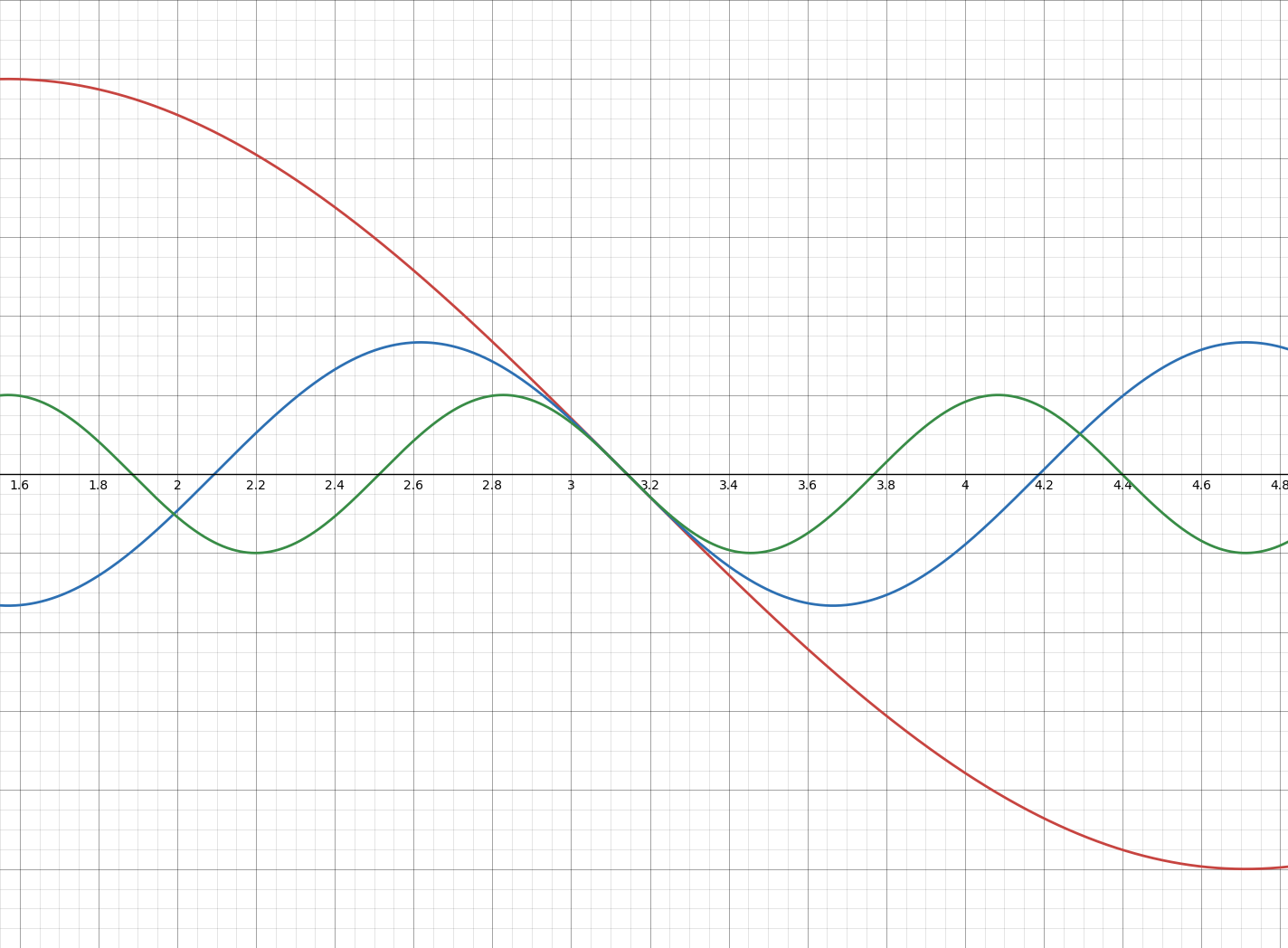
The first, third, and fifth sine harmonics crossing x equals pi from positive to negative. — Odd harmonics cross together at the sign change

The square wave itself flips sign halfway through its period, so we want sine waves that also flip sign after shifting by $\pi$ . Notice here that all of the odd harmonics go across $x=\pi$ from top to bottom, which does not hold for even harmonics. So, in order to constructively help make the square wave, we omit the even harmonics and stick to odd. If you are wondering why this is true, notice that for $\sin(kx)$ , shifting by $\pi$ gives $\sin(k(x+\pi))=(-1)^k\sin(kx)$ . Odd $k$ terms flip sign, matching the square wave's half-period sign flip, while even $k$ terms do not.

Now, let us generalize the approximation:

S_N(x)=\frac{4}{\pi}\sum_{n=1}^{N}\frac{\sin((2n-1)x)}{2n-1}

And take $N$ to infinity.

The eleventh Fourier partial sum for the square wave. — $S_{11}(x)$

The twenty-fifth Fourier partial sum for the square wave. — $S_{25}(x)$

The ninety-ninth Fourier partial sum for the square wave. — $S_{99}(x)$

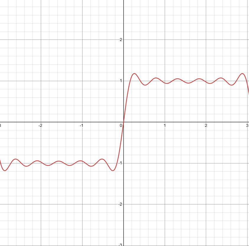
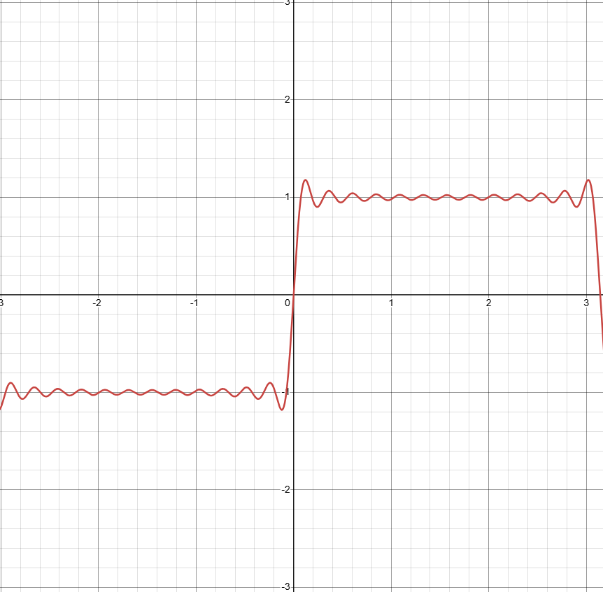
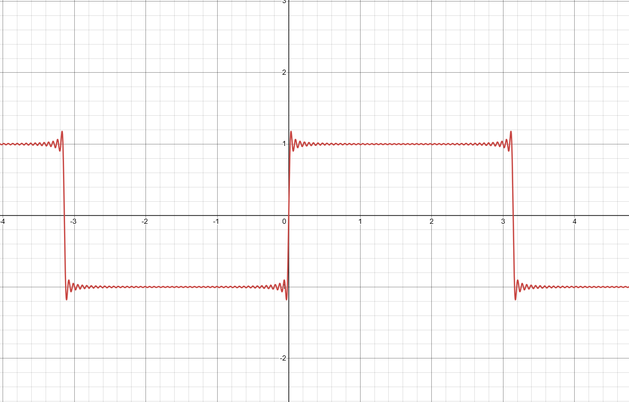
Beautiful. We have just recreated the square wave by summing sine waves. Notice that the low frequency sine waves give rise to the broad structure, and the high frequency waves give the tiny corrections. However, since all of the odd harmonics cross zero with the same behavior, they complement each other and create the overall "on and off" behavior we were looking for.

Notice something interesting in the images: the square wave approximations overshoot the discontinuities slightly. This is known as the Gibbs phenomenon. It is not a bug in Desmos or a numerical error. Essentially, we are trying to create a sharp vertical jump with smooth sine waves. So, there must be a slight bump since sine cannot perfectly snap into place. As $N$ increases, the overshoot bump gets thinner, but it stays the same height. In fact, the height approaches a fixed size of about 9% of the jump.

It is also important to note that the $\frac{4}{\pi}$ included in the series is important to normalize the function. Without the coefficient, the odd-harmonic sine sum converges to $\frac{\pi}{4}$ on the positive plateau. To scale the wave to jump between $1$ and $-1$ , we multiply by $\frac{4}{\pi}$ . Once you realize a wave is controlled by its frequency recipe, the natural next move is to start changing this recipe.

Changing The Recipe

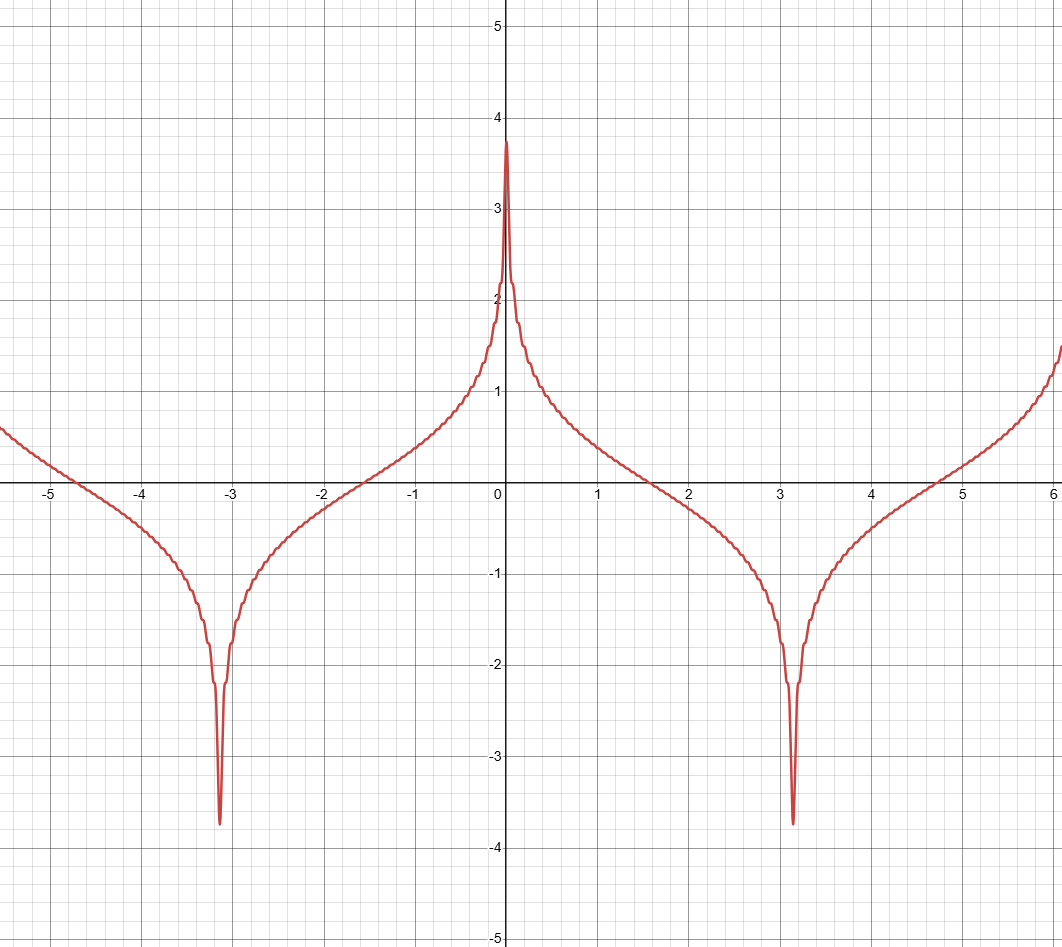
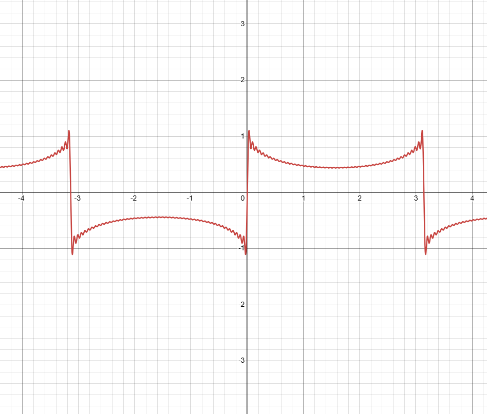
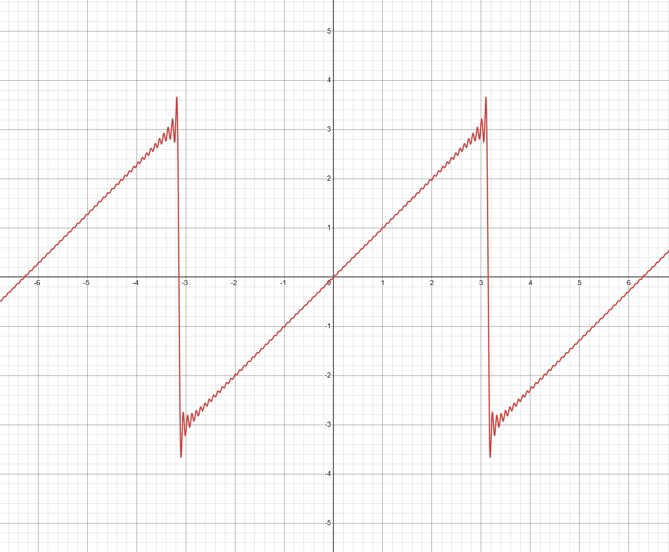
We have accomplished our original goal of recreating the square wave. But there are plenty of other questions to be asked. For example, what happens if we use even harmonics instead? What about the other trigonometric functions? It turns out, you can make a bunch of very interesting waves with this same approach. Here are some of my favorites:

C_N(x)=\sum_{n=1}^{N}\frac{\cos((2n-1)x)}{2n-1}

Cosine with odd harmonics plotted on a coordinate grid. — Cosine with odd harmonics

G_N(x)=\sum_{n=1}^{N}\frac{\sin((2n-1)x)}{2n}

A sine series using odd harmonics with even coefficients in the denominator. — Sine with odd harmonics inside sine but even coefficients in the denominator

f_N(x)=2\sum_{n=1}^{N}(-1)^{n+1}\frac{\sin(nx)}{n}

A sawtooth wave approximation plotted on a coordinate grid. — known as Sawtooth wave

Part 2

Applications in Electronics

In the first section, we built a square wave with smooth sine waves. While this is surprising, it is not the overarching idea behind Fourier approximations, especially in electronic signaling.

The overarching idea is actually the other way around: complicated signals can be broken down into frequency components. This is where Fourier approximations can become less math and more physics and engineering.

Let us start in the digital world. Here, a transmitter usually sends information to a receiver by switching between 0s and 1s: 0 is low voltage, and 1 is high voltage. A clean way to transmit this information would be with a square wave. The highs would represent 1s, and the lows would represent 0s. This is what would take place in a perfect, idealized digital world.

Physically, however, something very different is happening. These electrical signals interact with conductors, face capacitance and resistance, interact with noise, and much more. In reality, a signal can never be transmitted perfectly to another device. Digital information is discrete in theory but analog in reality. This creates a new way to interpret the square wave from earlier.

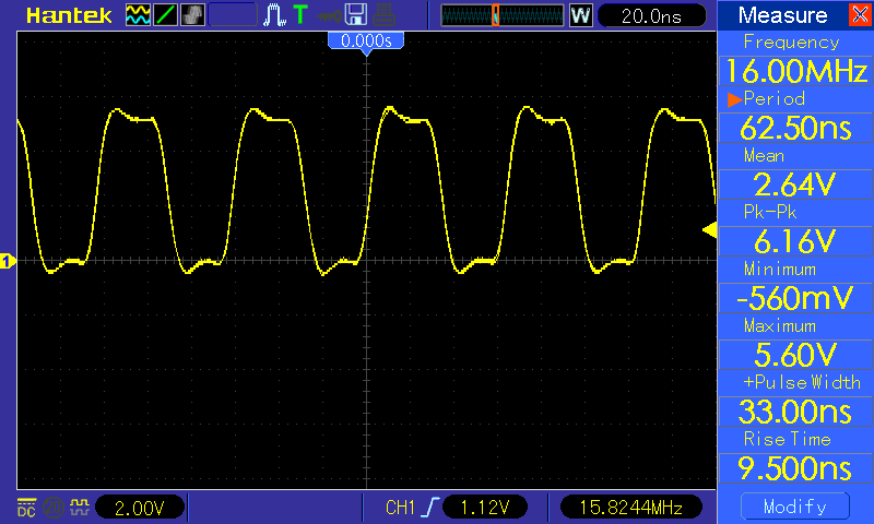
From the first section, we know that the square wave's general shape is made from low frequencies, while high frequencies sharpen it out. However, due to real conditions, the higher frequencies can get weakened, distorted, or reflected. According to our approximations, a square wave without the high frequencies would appear rounded and not very discrete.

This idea is known as bandwidth. Bandwidth is the range of frequencies that are able to be transmitted to another device. Ideally, infinite bandwidth would help us produce perfect square waves at the receiver. But in reality, the square waves can appear flat and smoothed out.

To sum up so far, signals can be broken down into frequency components. However, because of real conditions like capacitance, resistance, and noise, higher frequencies can be distorted. Thus, square waves are going to appear more smooth and rounded than an ideal square wave.

At low clock speeds, this low bandwidth is okay, since the waves have enough time to rise and fall and thus be processed. However, at high clock speeds, this can make or break a system. If a smoothed-out wave does not have enough time to drop before another wave comes in, the receiver cannot tell when the lows and highs actually happened.

So, how does one increase bandwidth? You can start by reducing what caused reduced bandwidth in the first place. That means reducing capacitance, reducing length, having less resistance/impedance to interact with, and using stronger drivers that change voltage more quickly.

In this whole blog post, we have learned how signals are approximated using sums of frequencies, and how the applications of this helped us learn the limitations of signals using bandwidth, as well as how to reduce those limitations.

The deeper lesson is not just that sine waves can build a square wave. It is that shape can be understood through frequency. Once a signal is described by its frequency recipe, questions about noise, filtering, bandwidth, and compression become much more natural. This is where Fourier series stops feeling like a trick and starts feeling like signal processing.

Oscilloscope capture of a low bandwidth square wave with rounded rising and falling edges. — Low bandwidth square wave. Image adapted from Electronics Stack Exchange user Zhenek, licensed under CC BY-SA. Source: Electronics Stack Exchange.

Sources / Further Reading

Daniel A. Russell's Fourier Synthesis of Periodic Signals, Keysight's oscilloscope bandwidth note, and the standard reference on the Gibbs phenomenon.