Autonomous equations
#051
Problem
Classification
- growth
- equilibrium
- autonomous
Method
- separable
Solution
Simulation & Code
Computational workSimulation
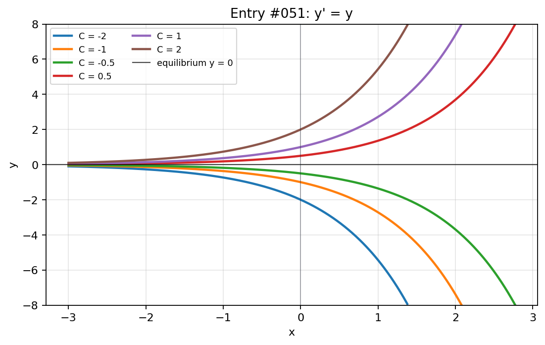
Python codeOpen
import numpy as np
import matplotlib.pyplot as plt

x = np.linspace(-3, 3, 600)
constants = [-2, -1, -0.5, 0.5, 1, 2]

fig, ax = plt.subplots(figsize=(7, 4.5))

for constant in constants:
    y = constant * np.exp(x)
    y = np.where(np.abs(y) <= 8, y, np.nan)
    ax.plot(x, y, linewidth=2, label=f"C = {constant}")

ax.axhline(0, color="black", linewidth=1, alpha=0.7, label="equilibrium y = 0")
ax.axvline(0, color="#111827", linewidth=0.8, alpha=0.35)
ax.set_title("Entry #051: y' = y")
ax.set_xlabel("x")
ax.set_ylabel("y")
ax.set_ylim(-8, 8)
ax.grid(True, alpha=0.3)
ax.legend(fontsize=8, ncols=2)

fig.tight_layout()
plt.show()
Handwritten derivation
Download full PDFTakeaway & Interpretation
This is the basic exponential growth equation. The slope is proportional to the current value of y, so positive solutions grow upward and negative solutions move farther downward. The equilibrium y=0 is unstable because nearby nonzero solutions move away from it.